
What is this project about?
An end-to-end code solution with R. The objective of this project is to perform data cleansing, select an item from the database, conduct Exploratory Data Analysis (EDA), forecast sales using time series analysis in R with diverse machine learning models, and assess their performance using accuracy metrics. GitHub link
- Summary:
In this data, a seasonal effect was identified in EDA analysis. Among the forecasting models, the ARIMA model was selected as the superior choice due to its more favourable accuracy validation results.
rm(list = ls())

## Libraries----
library(fpp3)
library(GGally)
library(ggfortify)
library(fable)
library(forecast)
library(zoo)
library(xts)
library(dplyr)


## Set working directory----
# Set the working directory to the folder containing the CSV file
setwd("C:/test_input/")

##Load, Cleaning & Merge----
#Load the CSV file with ';' as the delimiter
sales_data <- read.csv("sales_data.csv", sep = ";") #file with sales data
store_master <- read.csv("store_master.csv", sep = ";") #file with stores data

#Fixing characters in latitude & longitude using gsub()
store_master <- store_master %>%
mutate(latitude = gsub(",", ".", latitude))
store_master <- store_master %>%
mutate(longitude = gsub(",", ".", longitude))

####Merge datasets ----
#merge imported and modified datasets and create a df with sales and store

sales_store <- left_join(sales_data, store_master, by = "store")
sales_store <- sales_store %>%
mutate(unit_price = gsub(",", ".", unit_price))

#change class of items, stores and categories to character from numeric to characters
#because they are categorical values
sales_store <- sales_store %>%
mutate(store = as.character(store)) %>%
mutate(item = as.character(item)) %>%
mutate(item_category = as.character(item_category))%>%
mutate(unit_price = as.numeric(unit_price)) %>%
mutate(date = as.Date(date))
———
Selecting ITEMs to forecast
10 items with the most available historical records have been considered for analysis
Group the data by ‘item’ and count the number of unique ‘date’ records for each item
item_counts <- sales_store %>%
group_by(item) %>%
summarise(date_count = n_distinct(date)) %>% arrange(desc(date_count))

selected_10_items <- as.list(head(item_counts[1], 10))
selected_10_items <- as.numeric(selected_10_items$item)

item_list = selected_10_items #selected items

# create tsibble for selected items & aggregate 'qty' and 'unite_price' by 'date'
# calculate 'total_qty' and 'unit_price' value for each item per day
## ITEM 1 -------------------------
### EDA----
item_1_df <- sales_store %>% #filter sales_store to get item specific data
filter(item == item_list[1], date >= as.Date("2017-01-01") & date <= as.Date("2019-12-31"))
item_1_df <- item_1_df %>% #arrange in desc order
arrange(item_1_df, desc(date))
#using aggregate functions for items, get the sum of 'qty' and mean for 'unit_price' in each day
sum_qty_df_item1 <- item_1_df %>%
group_by(date) %>%
summarise(total_qty = sum(qty), unit_price = mean(unit_price))
#head(sum_qty_df_item1) # View the new dataframe
tsibble_item1<- as_tsibble(sum_qty_df_item1, index = date) #convert to tsibble
# Sales plot for this item
p1_qty <-autoplot(tsibble_item1, .vars = total_qty) + labs(title = "Item 1")
p1_qty
 tsibble_item1 %>% #fix the class of date and identify index
mutate(date = as_date(date)) %>%
as_tsibble(index = date)
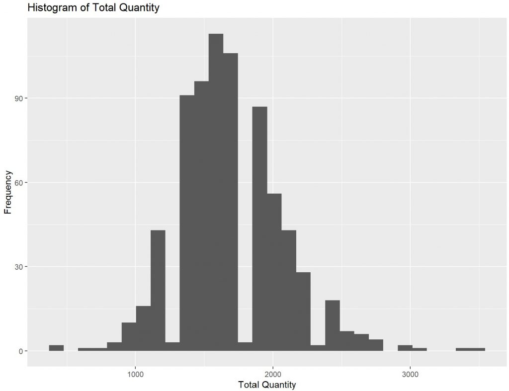
#### Histogram----
#Check histogram for 'total_qty' and 'unit_price'
hist1 <- ggplot(data = tsibble_item1, aes(x = total_qty)) +
geom_histogram() +
labs(x = "Total Quantity", y = "Frequency", title = "Histogram of Total Quantity")
hist1
tsibble_item1 %>% #fix the class of date and identify index
mutate(date = as_date(date)) %>%
as_tsibble(index = date)
#### Histogram----
#Check histogram for 'total_qty' and 'unit_price'
hist1 <- ggplot(data = tsibble_item1, aes(x = total_qty)) +
geom_histogram() +
labs(x = "Total Quantity", y = "Frequency", title = "Histogram of Total Quantity")
hist1
 #### Correlogram----
ts_data_item1 <- tsibble_item1 %>%
as_tsibble(index = date) %>%
fill_gaps()
acf_1_lag365 <- ts_data_item1 %>%
ACF(total_qty, lag_max = 365) %>% autoplot()
acf_1_lag365
#### Correlogram----
ts_data_item1 <- tsibble_item1 %>%
as_tsibble(index = date) %>%
fill_gaps()
acf_1_lag365 <- ts_data_item1 %>%
ACF(total_qty, lag_max = 365) %>% autoplot()
acf_1_lag365
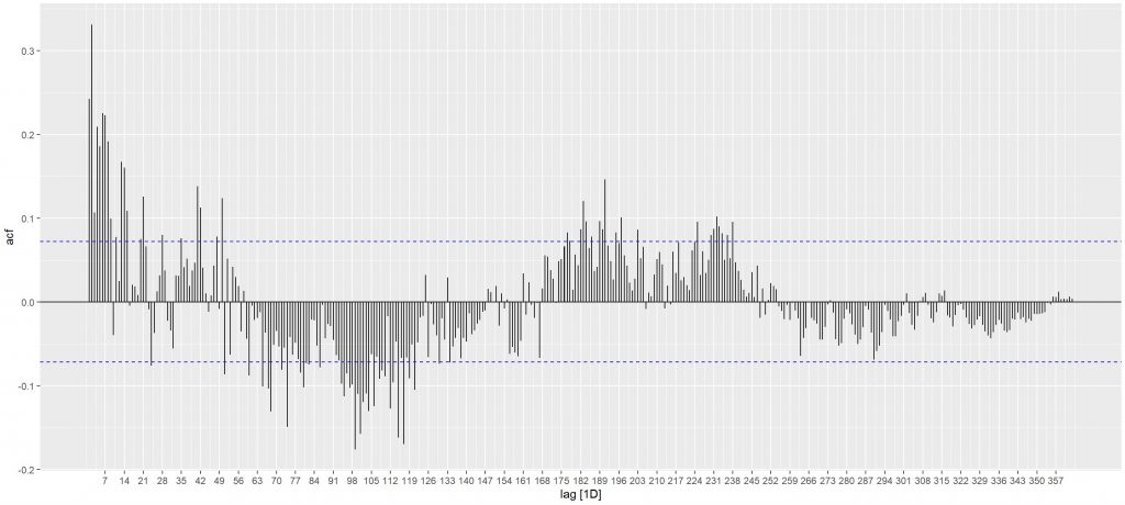
There is a seasonal pattern according to ACF.
The variable “total_qty” shows a statically significant correlation with the most recent observed data, suggesting that forecasting methods that rely on recent observations tend to yield better results. Additionally, there is a noticeable seasonal pattern on the weekly dataframe.
#### Scatterplot---- #study correlation between 'unit_price' and 'total_qty' scatter_plot1 <- tsibble_item1 %>% ggplot(aes(x=total_qty, y=unit_price)) + geom_point() + labs(x = "Total Quantity for Item", y = "Unit Price") scatter_plot1#drop the 'price_unit' column and set index tsble_itm1_drpd <- tsibble_item1 %>% select(date, total_qty) %>% as_tsibble(index=date) #### Decomposition---- #additive decomposition because the magnitude of seasonal fluctuation does not vary with level tsble_itm1_drpd <- tsble_itm1_drpd %>% # fill gaps as_tsibble(index = date) %>% fill_gaps() dcmp_item1 <- tsble_itm1_drpd %>% mutate(total_qty = na.aggregate(total_qty, FUN = median)) %>% model(stl = STL(total_qty)) #components(dcmp_item1) autoplot(components(dcmp_item1))
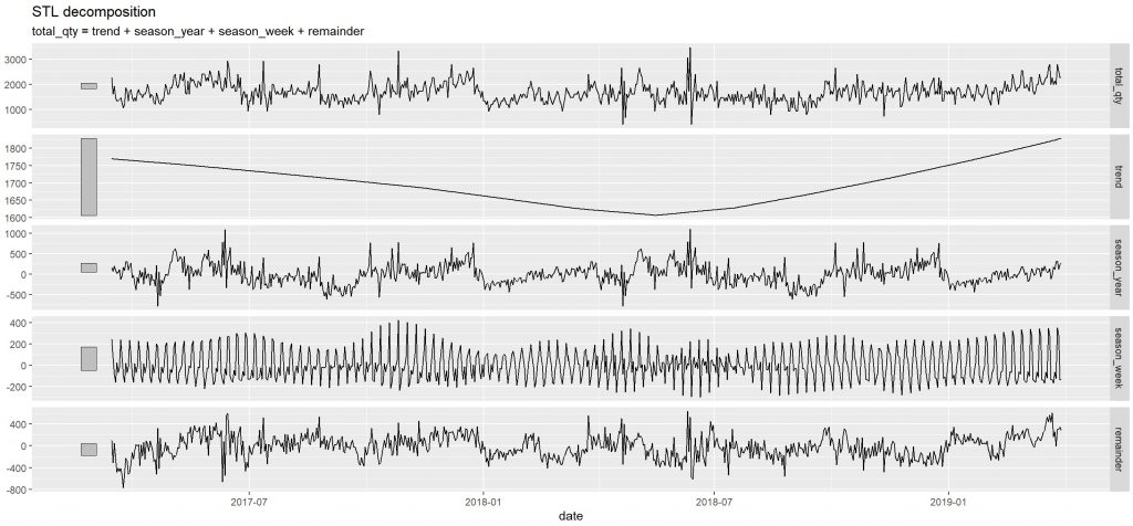
STL decomposition depicts both positive and negative trend in the data. The trend has a relatively small magnitude in both direction.
###Forecast -------------------------------------------
####converting data to ts-----
##Creating xts object and fixing missing date values
tsble_itm1_drpd_xts <- xts(tsble_itm1_drpd$total_qty, tsble_itm1_drpd$date)
start_date_item1 <- first(tsble_itm1_drpd$date) #find start date
end_date_item1 <- last(tsble_itm1_drpd$date) #find end date
##create a seq of dates in order, without missing date value
dates_xts_item1 <- seq(as.Date(start_date_item1), as.Date(end_date_item1), by="days")
##convert to date df and merge them by left join to add all probable missing date values
##convert dates to df
df_temp_1_1 <- as.data.frame(dates_xts_item1)
colnames(df_temp_1_1) <- "date"
##merge, interpolate NA values & conversions
df_temp_1_2 <- as.data.frame(tsble_itm1_drpd)
df_dates_merged_item1 <- left_join(df_temp_1_1, df_temp_1_2, by = "date")
xtsdates_merged_item1 <- xts(df_dates_merged_item1$total_qty, df_dates_merged_item1$date)
xtsdates_merged_item1 <- na.approx(xtsdates_merged_item1)
##conversions for date, create ts and break date to YYYY, MM, DD
date_obj_item1_1 <- as.Date(start_date_item1)
year <- as.numeric(format(date_obj_item1_1, "%Y"))
month <- as.numeric(format(date_obj_item1_1, "%m"))
day <- as.numeric(format(date_obj_item1_1, "%d"))
startdate_for_ts1 <- c(year, month, day) #start date as vector
date_obj_item1_2 <- as.Date(end_date_item1)
year <- as.numeric(format(date_obj_item1_2, "%Y"))
month <- as.numeric(format(date_obj_item1_2, "%m"))
day <- as.numeric(format(date_obj_item1_2, "%d"))
##time-series for item
enddate_for_ts1 <- c(year, month, day) #end date as vector
ts_item1 <- ts(xtsdates_merged_item1, frequency = 365, start =startdate_for_ts1, end = enddate_for_ts1)
####Define test and train sets----
test_no_item1 <- round(nrow(ts_item1)*0.2)
test_item1 <- tail(ts_item1, test_no_item1) #20% of last obs as test
train_no_item1<- round(nrow(ts_item1))-test_no_item1
train_item1<- head(ts_item1, train_no_item1) #80% of first obs as train
####Fit models ----
###ARIMA
fit1_arima <- auto.arima(train_item1) %>%
forecast(h = test_no_item1)
###SARIMA
p <- 1 # AR order -- The model uses the previous value as a predictor bc of ACF
d <- 0 # Differencing order -- bc the plot is close to stationary the original data is assumed to be already stationary. if there is no significant trend, d can be set to 0
q <- 1 # MA order -- It represents the number of lagged forecast errors (residuals) to include in the model
P <- 1 # Seasonal AR order -- indicating that the model includes the lagged value of the seasonal component
D <- 1 # Seasonal differencing order -- When the time series shows clear seasonality D can be set to a positive value
Q <- 1 # Seasonal MA order, model includes the lagged residuals of the seasonal component.
S <- 7 # Seasonal period (e.g.,7 for weekly seasonality)
fit1_sarima <- arima(train_item1, order = c(p, d, q), seasonal = list(order = c(P, D, Q), period = S)) %>%
forecast(h = test_no_item1) # Adjust the forecast horizon
###Snaive
fit1_snaive <- snaive(train_item1, h=test_no_item1)
###Mean
fit1_mean <- meanf(train_item1, h=test_no_item1)
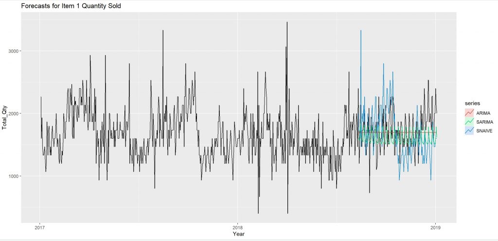
###PLOTS
plot_f1 <- autoplot(ts_item1) +
autolayer(fit1_snaive, series = 'SNAIVE', PI = FALSE) +
autolayer(fit1_sarima, series = 'SARIMA', PI = FALSE) +
autolayer(fit1_arima, series = 'ARIMA', PI = FALSE) +
xlab("Year") + ylab("Total_Qty") +
ggtitle("Forecasts for Item 1 Quantity Sold")
plot_f1
 ####Accuracy----
accuracy(fit1_snaive, test_item1)[2, c('RMSE', 'MAE')]
accuracy(fit1_sarima, test_item1)[2, c('RMSE', 'MAE')]
accuracy(fit1_arima, test_item1)[2, c('RMSE', 'MAE')]
####Accuracy----
accuracy(fit1_snaive, test_item1)[2, c('RMSE', 'MAE')]
accuracy(fit1_sarima, test_item1)[2, c('RMSE', 'MAE')]
accuracy(fit1_arima, test_item1)[2, c('RMSE', 'MAE')]
SARIMA model has been chosen for forecasting. This decision is based on several factors, including the fitness of the SARIMA model in capturing the patterns observed in the plot, as well as considering the error values. While the EMA model performs well, the SARIMA model is deemed to be a better fit overall for this particular analysis.
####BEST FORECASTS:
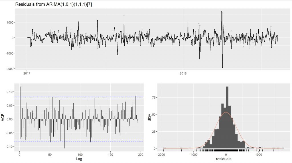
checkresiduals(fit1_sarima)
The p-value for the model’s residuals is larger than 0.05. This is considered good because it indicates that there is no significant correlation in the residuals at different lag values. Additionally, the histogram of the residuals closely resembles a normal distribution, which is desirable for a reliable model. Moreover, the residuals appear to exhibit characteristics of white noise, further supporting the goodness of the model. Based on these observations, it can be concluded that the model is performing well and is a good fit for the data.
####Estimated Values----

fit1_final <- arima(ts_item1, order = c(p, d, q), seasonal = list(order = c(P, D, Q), period = S)) %>%
forecast(h = 30)

####Table & Graph-----

plot(fit1_final, PI = FALSE)
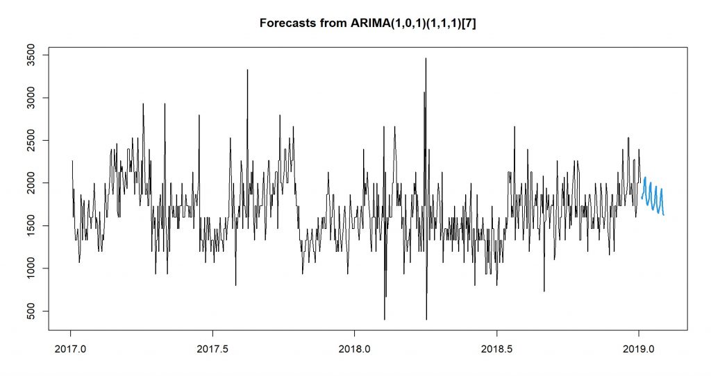
The prediction of sales for this item in the next 30 days.
# Extract the point forecasts from the forecast object
point_forecasts_1 <- as.numeric(fit1_final$mean)

# Determine the forecast horizon length
horizon_length <- length(point_forecasts_1)

##create a seq of dates in order for forecast data
dates_forecast1 <- seq(as.Date(end_date_item1) + 1, by = "day", length.out = horizon_length)

# Create a tsibble object using the point forecasts and dates
forecast_1_final <- tsibble(Date = dates_forecast1, Quantity = point_forecasts_1) %>%
mutate(Item = item_list[1])

autoplot(forecast_1_final) #plot final forecast
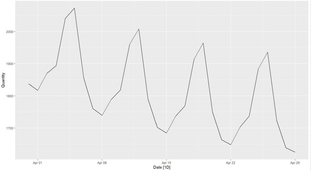
The plot for forecasted sales in 30 days.
print(forecast_1_final, n=30) #forecast values table

# A tsibble: 30 x 3 [1D]
   Date       Quantity  Item
   <date>        <dbl> <dbl>
 1 2019-03-31    1838.   385
 2 2019-04-01    1817.   385
 3 2019-04-02    1870.   385
 4 2019-04-03    1893.   385
 5 2019-04-04    2041.   385
 6 2019-04-05    2073.   385
 7 2019-04-06    1856.   385
 8 2019-04-07    1760.   385
 9 2019-04-08    1740.   385
10 2019-04-09    1789.   385
11 2019-04-10    1818.   385
12 2019-04-11    1960.   385
13 2019-04-12    2008.   385
14 2019-04-13    1791.   385
15 2019-04-14    1702.   385
16 2019-04-15    1684.   385
17 2019-04-16    1737.   385
18 2019-04-17    1769.   385
19 2019-04-18    1914.   385
20 2019-04-19    1964.   385
21 2019-04-20    1750.   385
22 2019-04-21    1663.   385
23 2019-04-22    1648.   385
24 2019-04-23    1703.   385
25 2019-04-24    1737.   385
26 2019-04-25    1884.   385
27 2019-04-26    1936.   385
28 2019-04-27    1723.   385
29 2019-04-28    1638.   385
30 2019-04-29    1624.   385